Model tuning

This page gives several examples about how to tune the model output towards observation.

The base example is given using the COVID-19 configuration of JUNE, the following parameters may be tuned:

• The number of people travel across super areas (e.g., group/commute/workplace_and_home.csv).

• Infection outcome (e.g., disease/infection_outcome.csv)

The experiments used to demostrate the tuning of model are described below:

Tuning information

Experiment name	Description	Location (only applicable at ESR)
Base	Base configuration with COVID-19	/tmp/june_realworld_auckland_base
Exp1	The multiplication factor for hospital/icu/home_ifr/hospital_ifr/icu_ifr = 10.0	/tmp/june_realworld_auckland_exp1
Exp2	The multiplication factor for contact frequency beta for all groups = 10.0	/tmp/june_realworld_auckland_exp2
Exp3	Increase maximum infectiousness 10.0 times more	/tmp/june_realworld_auckland_exp3
Exp4	Reduce the symptom cycle	/tmp/june_realworld_auckland_exp4

Base example

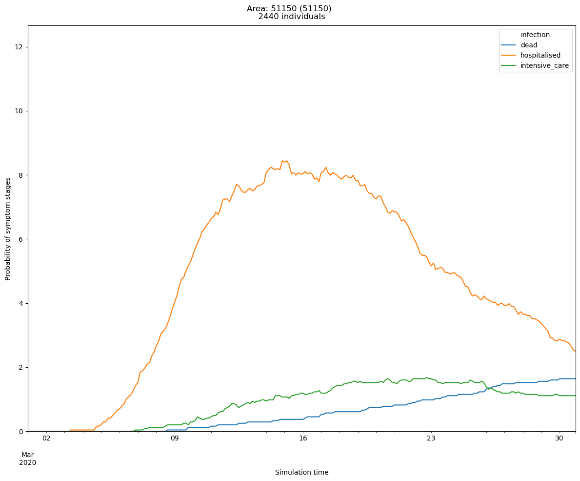
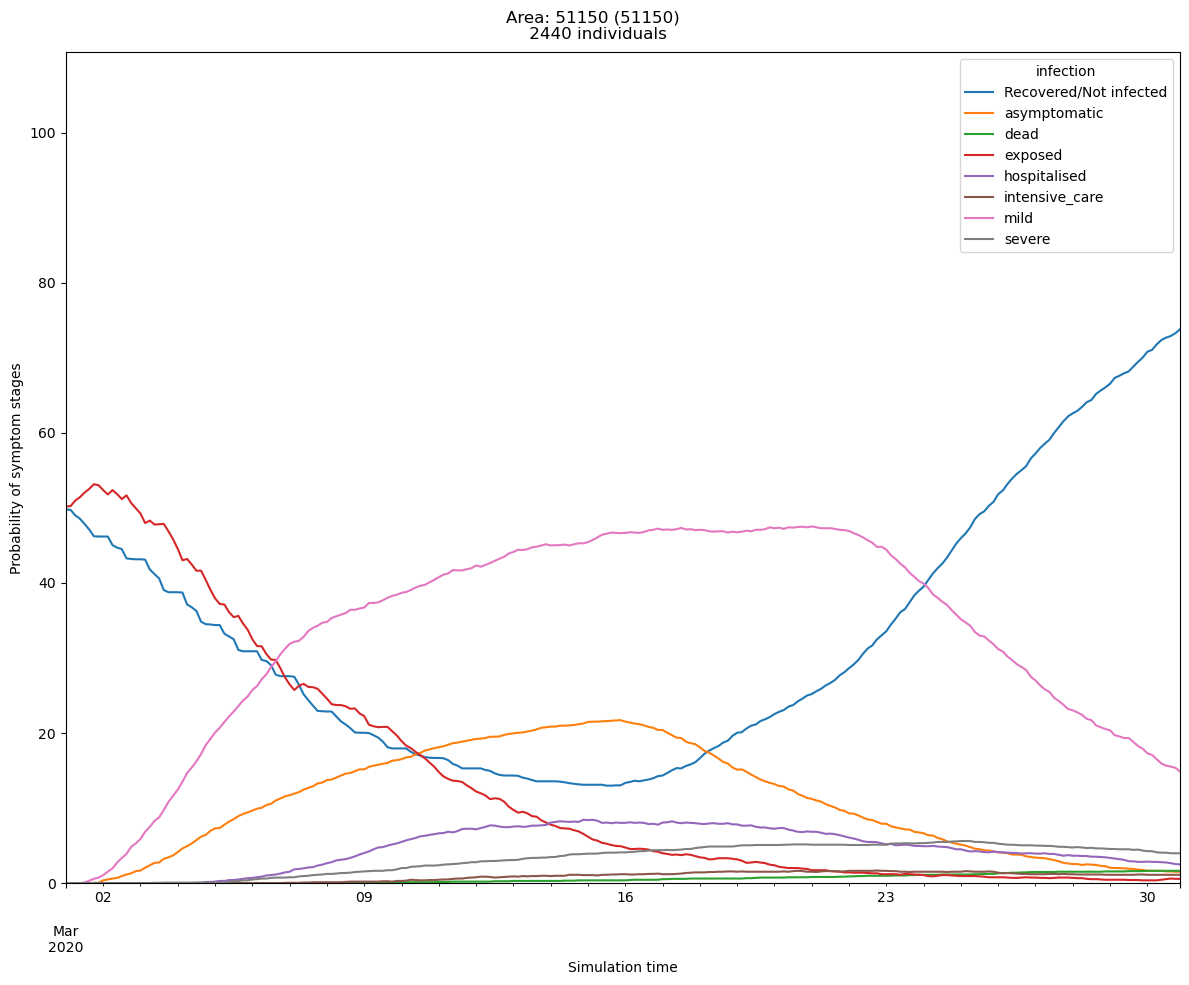
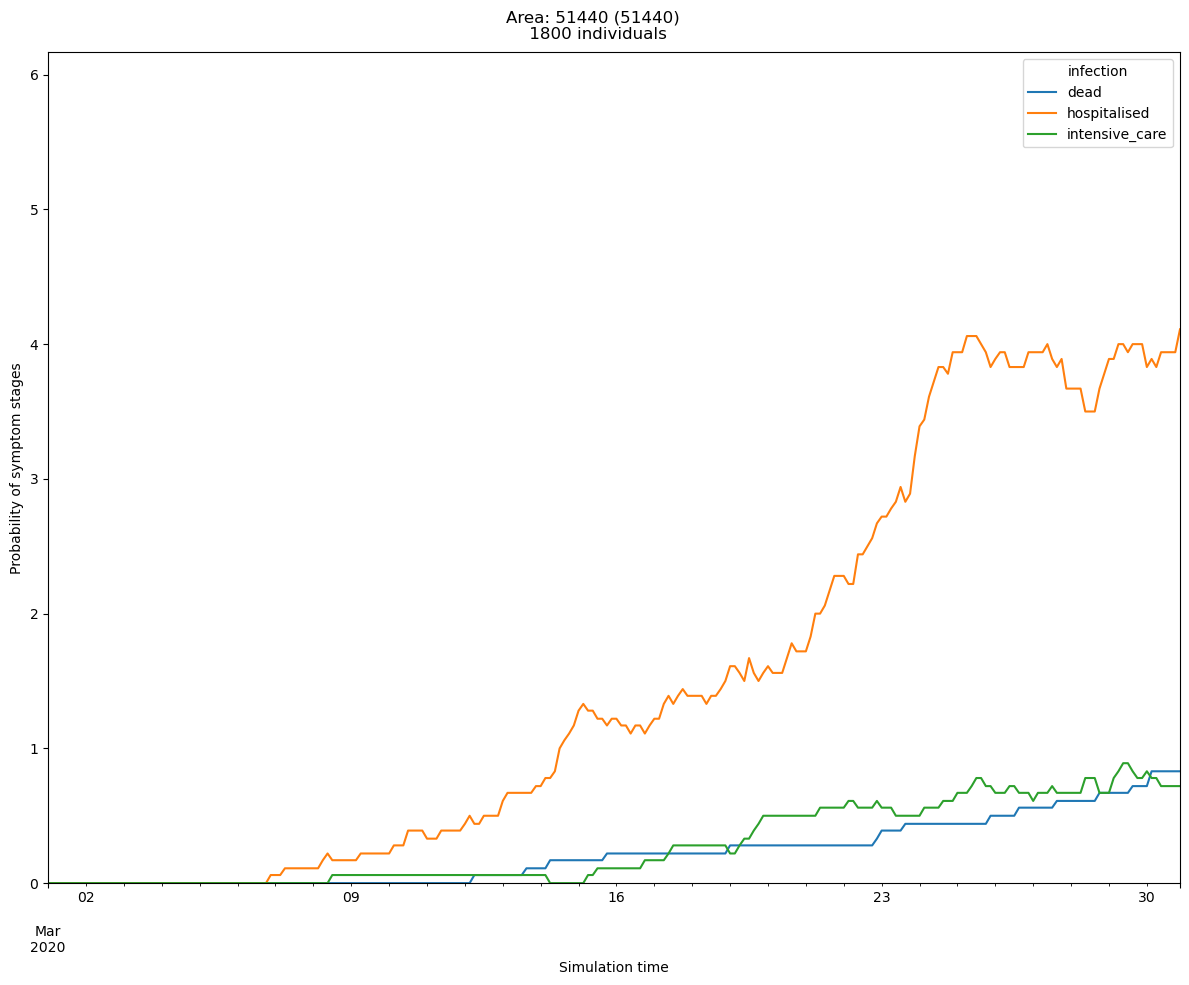
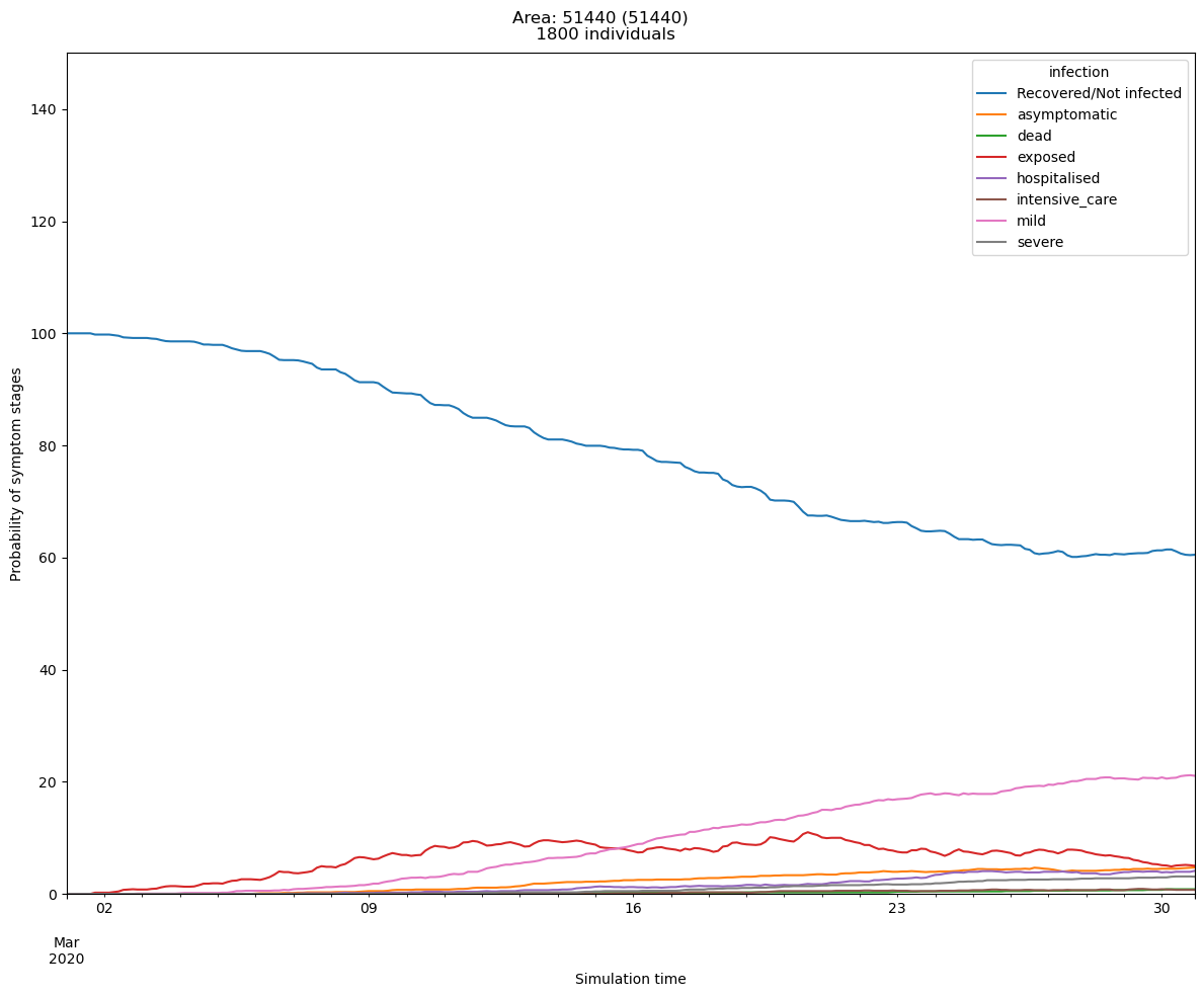
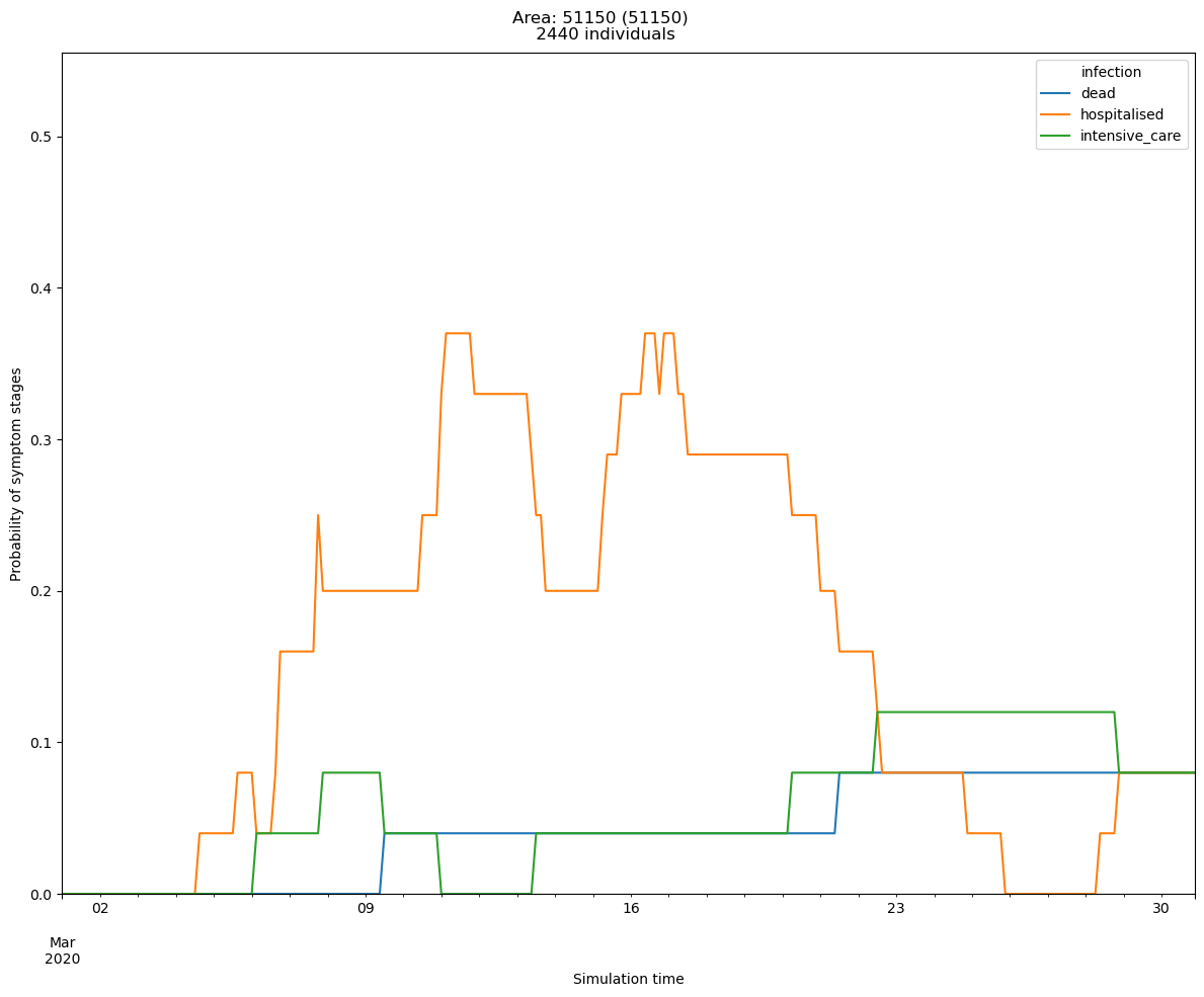
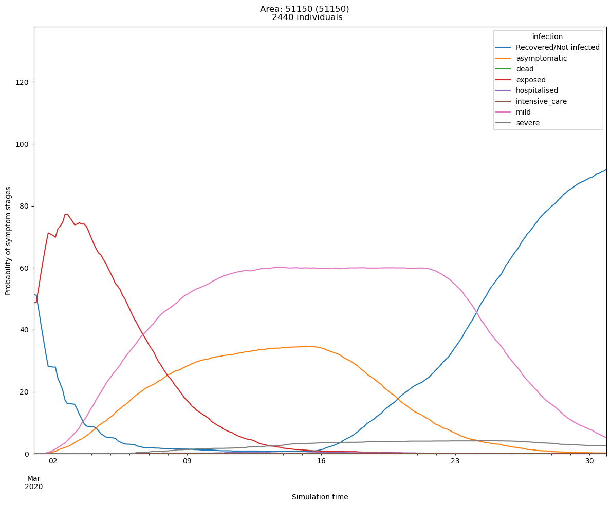
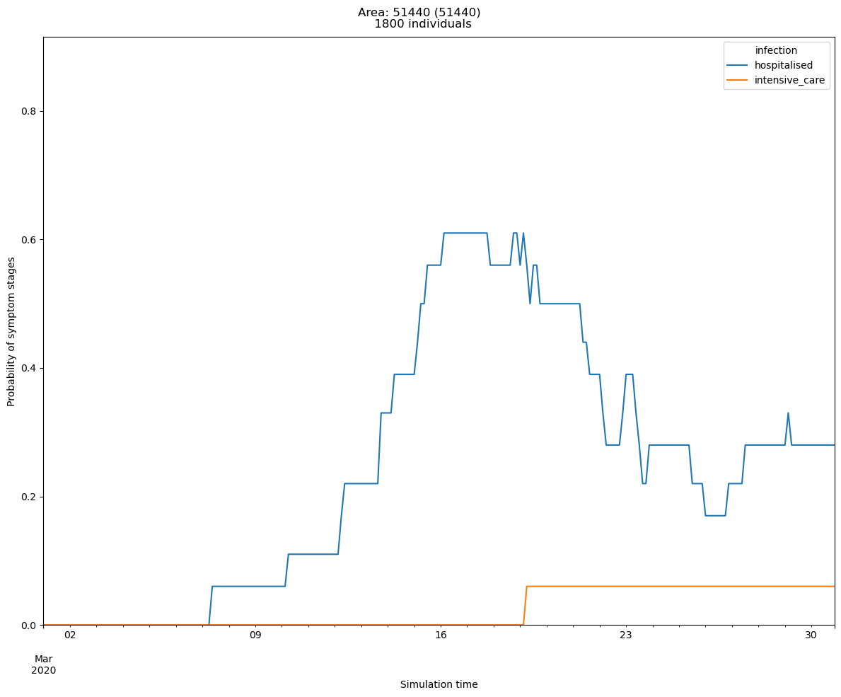
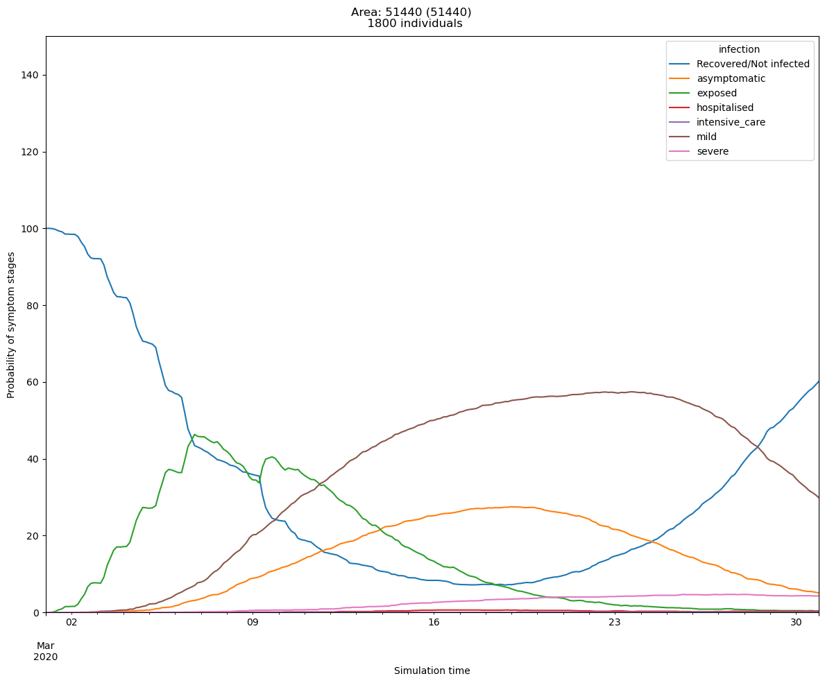
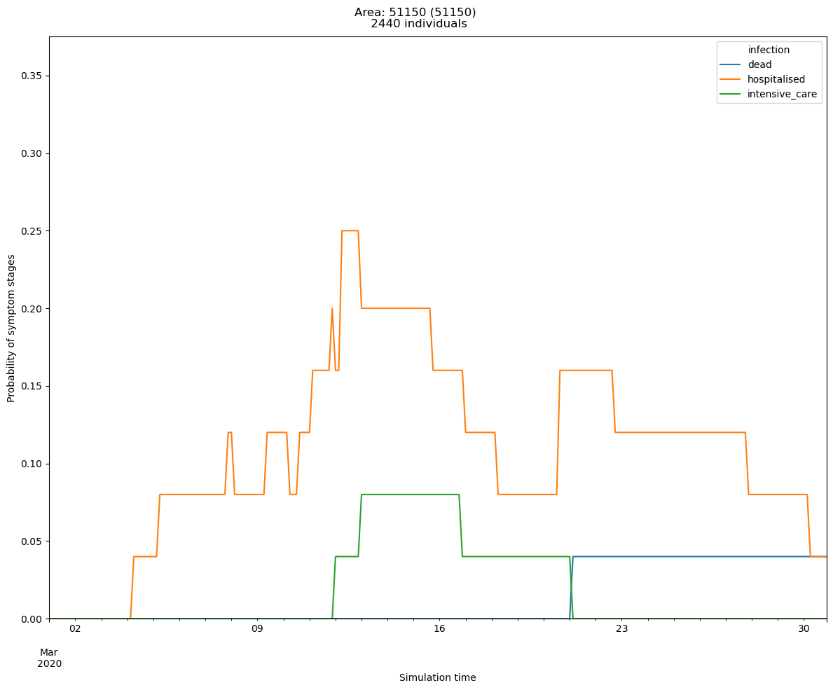
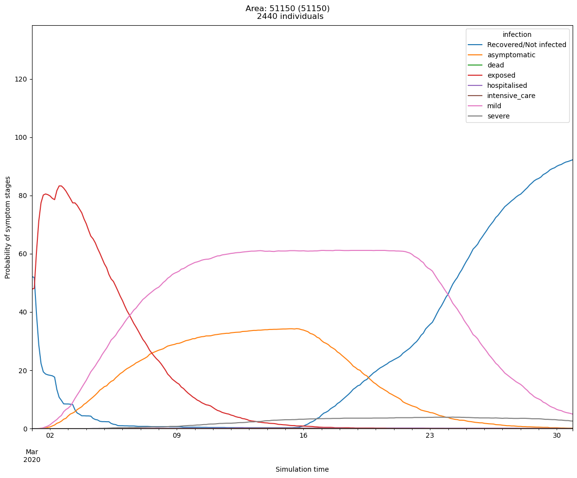
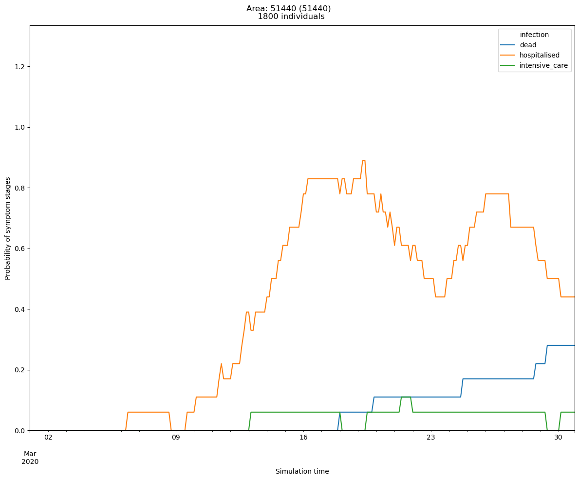
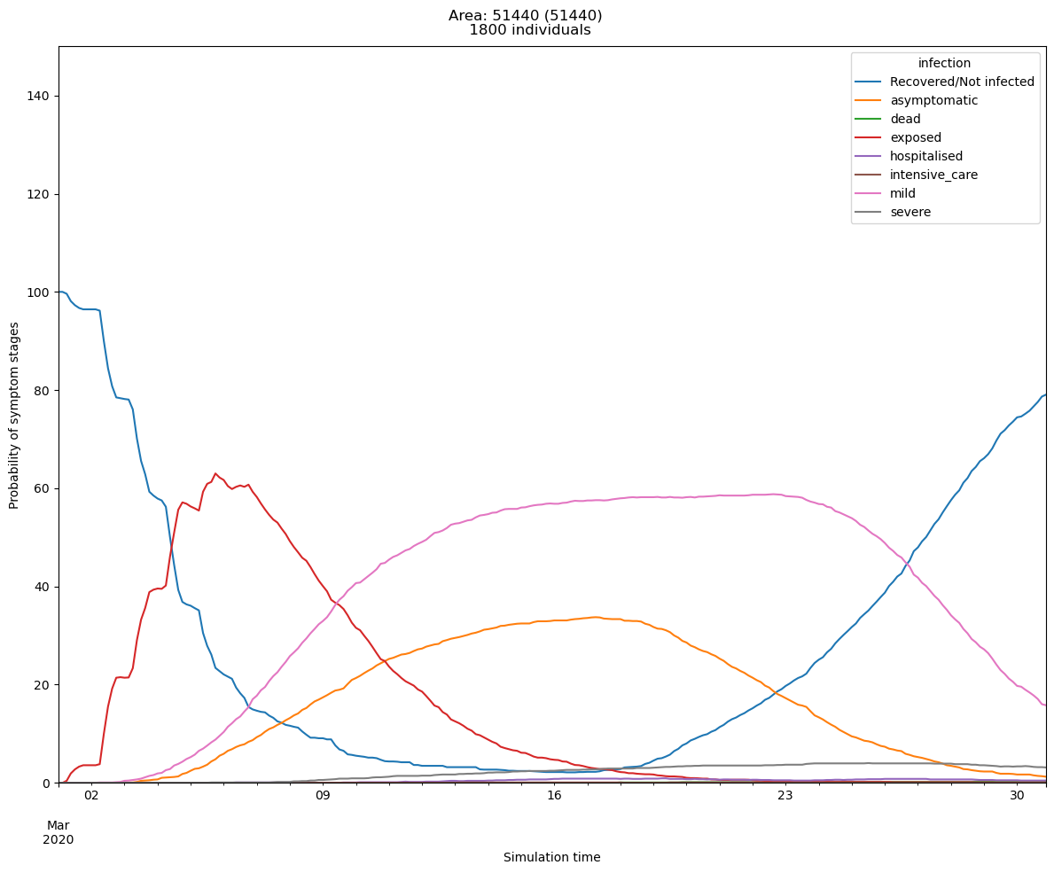
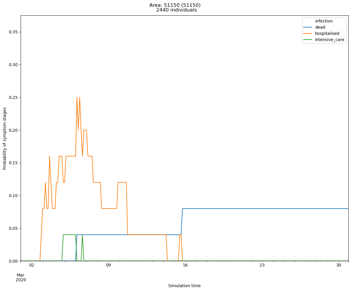
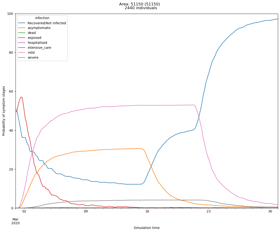
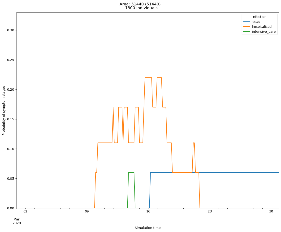
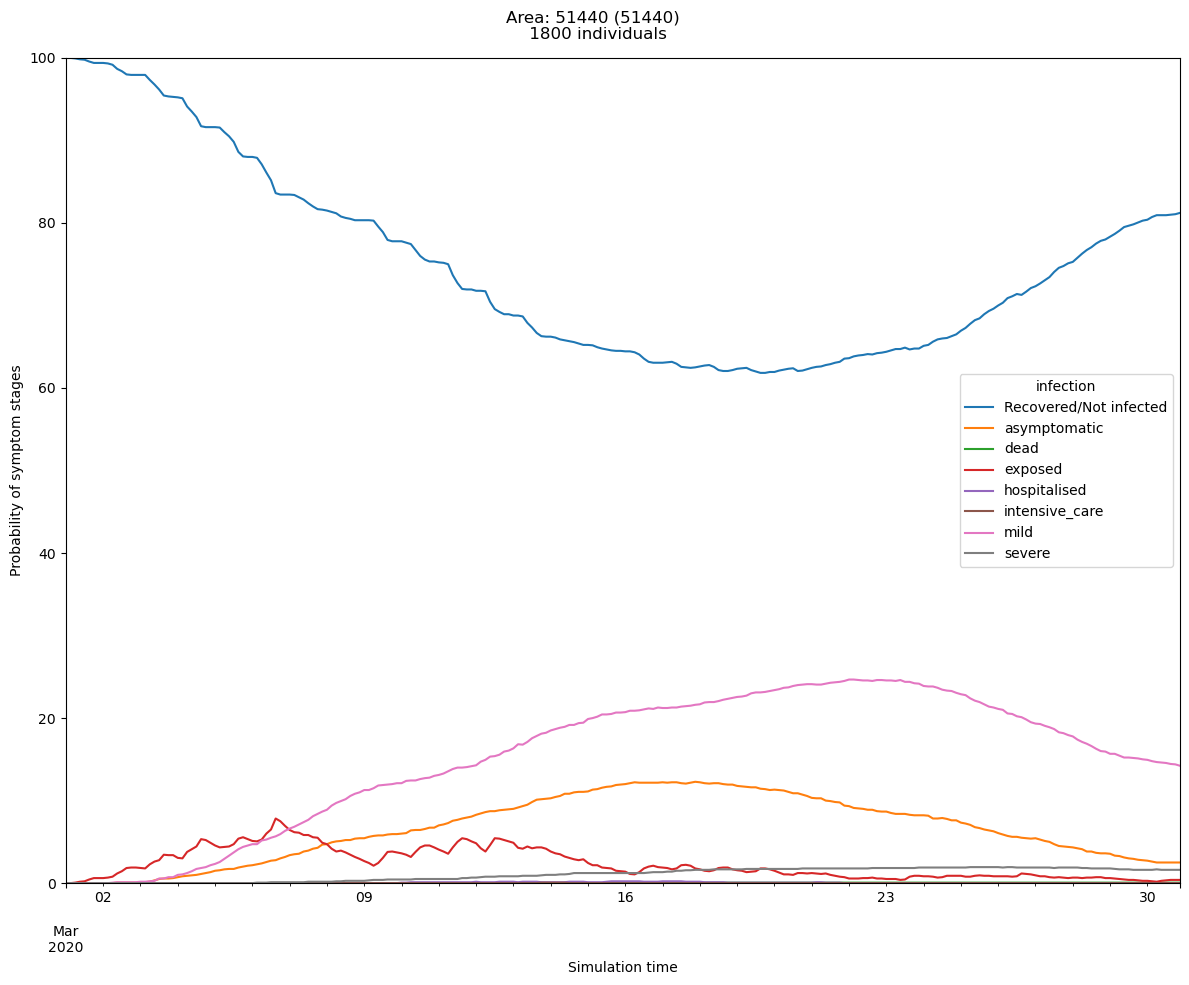
The base example is used to show the model outputs without any tuning. The following figures are the model outputs for the Area of 51150 and 51440.

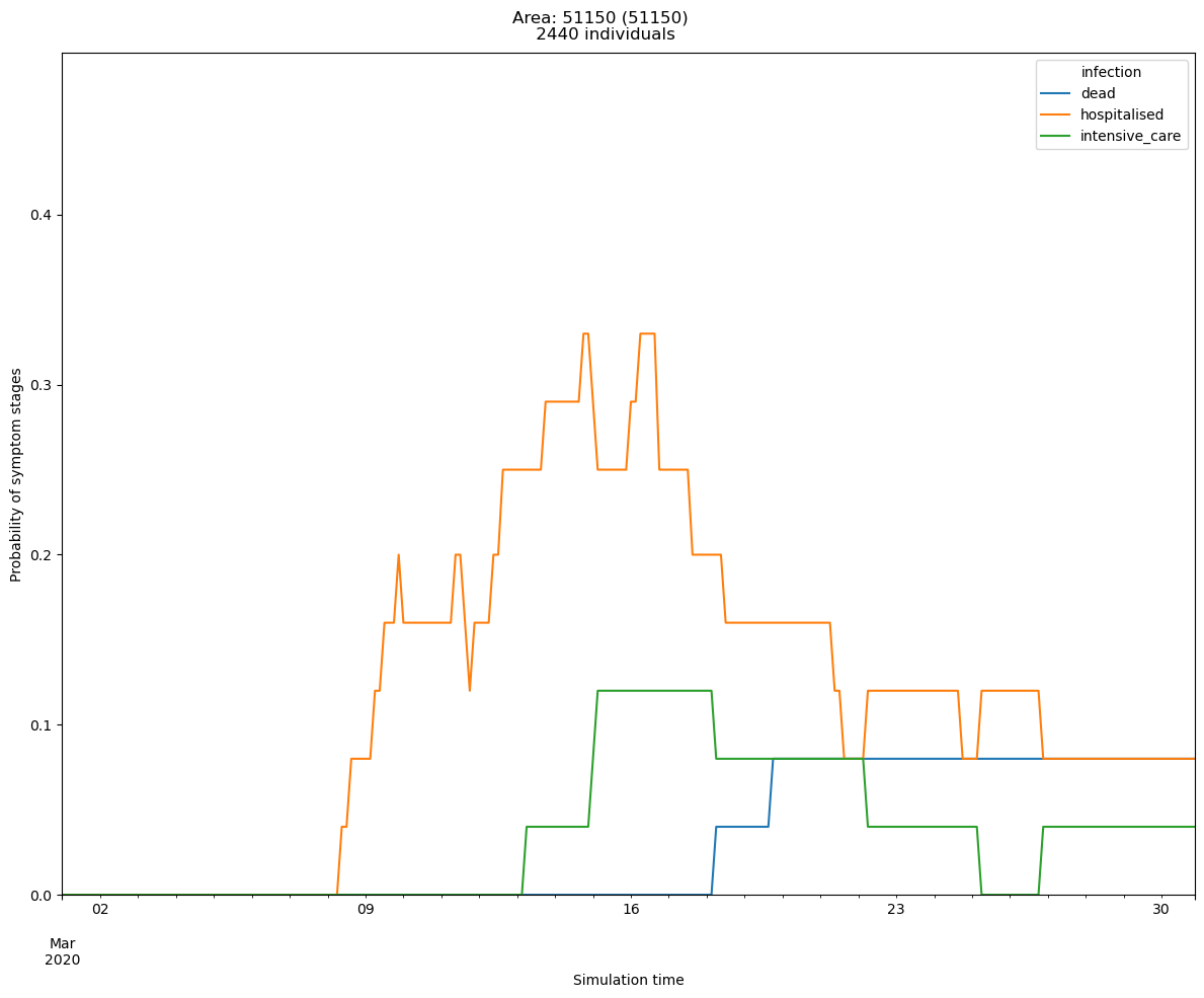
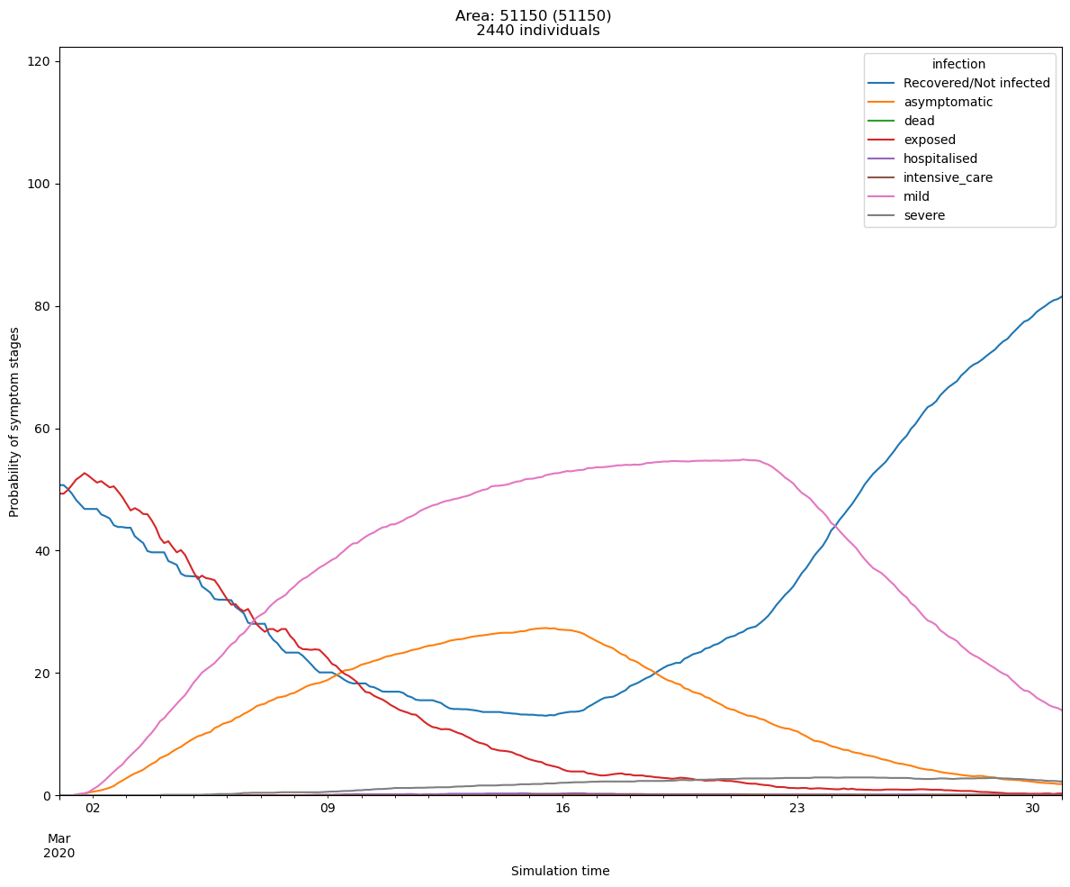
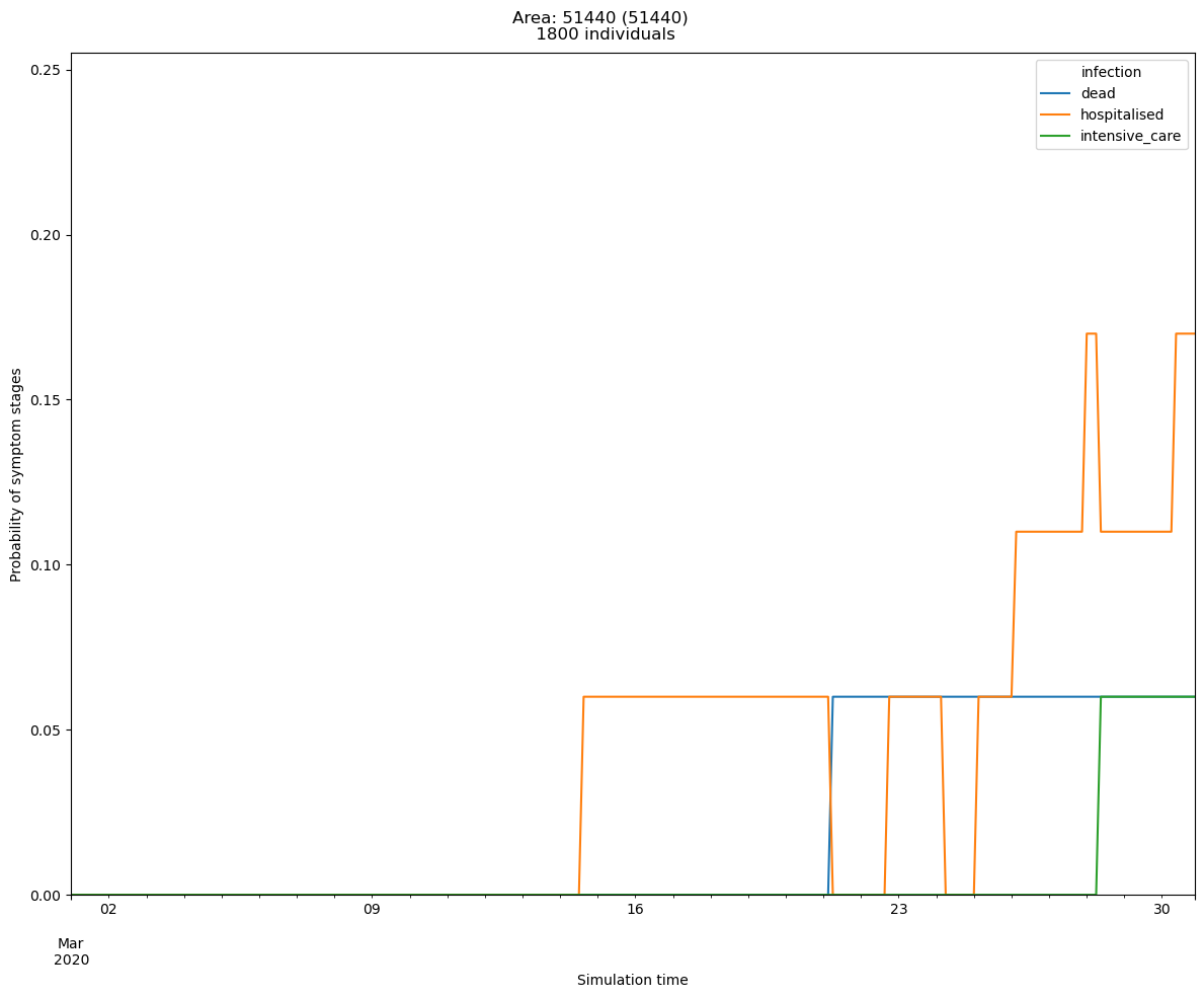
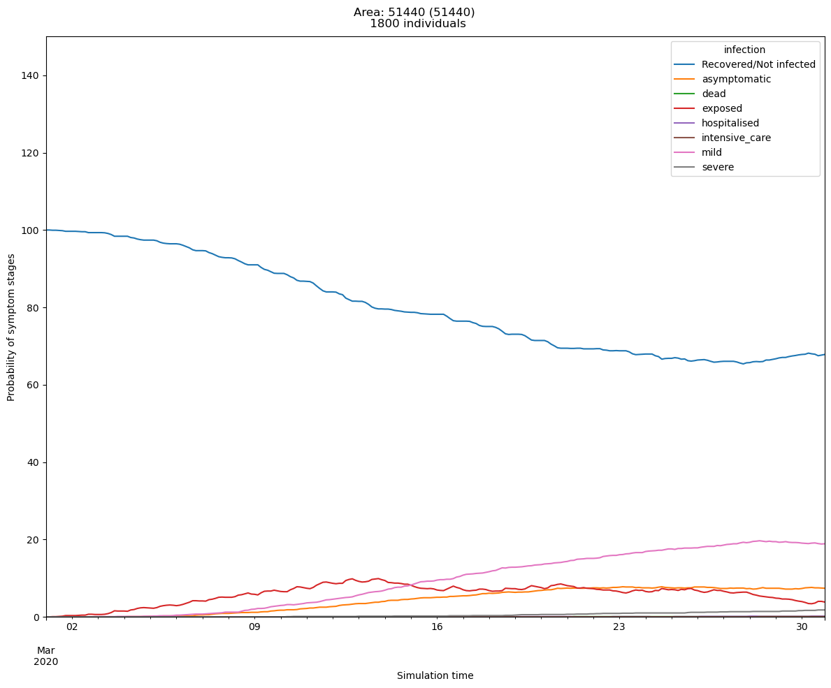
For 51150, we observe that the hospitalization rate was below 0.4%, indicating a relatively low proportion of individuals requiring hospital care. Conversely, the mortality rate stood at approximately 0.1%, suggesting a comparatively smaller percentage of individuals succumbing to the condition. It takes a while (e.g., 15 days) until we see the first hospital case in the Area 51440.

Increase the people is hospitalized and died

The number of people who died, were hospitalized, and placed into ICU can be increased by using the following configuration:

infection_outcome:
enable: true
adjust_factor:
   "18-65": # age range
      gp: # population type
      male: # sex
         asymptomatic: 1.0
         mild: 1.0
         hospital: 10.0
         icu: 10.0
         home_ifr: 10.0
         hospital_ifr: 10.0
         icu_ifr: 10.0
      female: # sex
         asymptomatic: 1.0
         mild: 1.0
         hospital: 10.0
         icu: 10.0
         home_ifr: 10.0
         hospital_ifr: 10.0
         icu_ifr: 10.0

In the case of 51150, there has been a significant increase in hospitalizations, rising from 0.4% to 8.0%. Similarly, the proportion of individuals requiring intensive care unit (ICU) treatment has increased from approximately 0.1% to 1-2%. Unfortunately, the mortality rate has also seen a rise, escalating from 0.1% to 1-2%.

Make people to be infected quicker

Increase contact frequency

The first apporach is that we can increase the contact frequency (\(beta\)) in etc/data/realworld_auckland/interaction/general.yaml:

contact_frequency_beta:
enable: true
adjust_factor:
   cinema: 10.0
   city_transport: 10.0
   company: 10.0
   grocery: 10.0
   gym: 10.0
   hospital: 10.0
   household: 10.0
   household_visits: 10.0
   inter_city_transport: 10.0
   pub: 10.0
   school: 10.0

As above, we increased the base contact frequency intensity by 10 times.

In comparison to the baseline experiment, a notable observation in Area 51150 is a higher rate of infection within the initial week. However, there haven’t been significant alterations in terms of hospitalization and mortality rates since the infection outcomes configurations were not modified.

On the other hand, the impact of the experiment is particularly pronounced in Area 51440. Here, the rate of infection has significantly accelerated when compared to the baseline experiment.

Change probability of infection

The probability of infection is determined by a Gamma function, which has three parameters: shape, scale and shift:

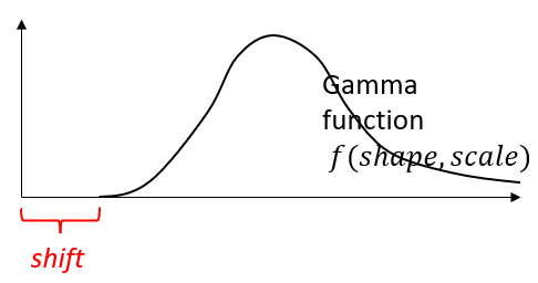
The probability of infection is considered from the moment a person is infected.

• The shift parameter determines the starting time of infection. Prior to the specified shift, the probability of infection is 0.0%.

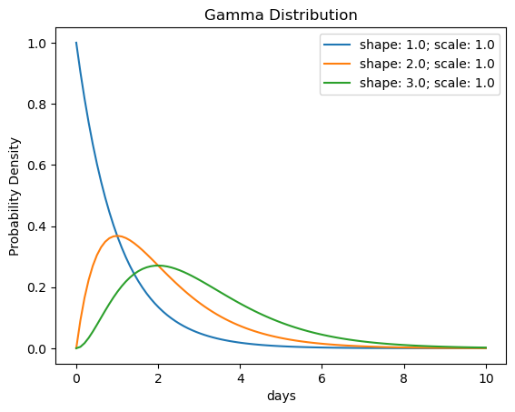
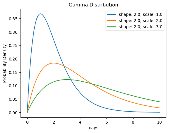
• On the other hand, the shape parameter defines the shape of the Gamma function, which influences the rate at which infectiousness reaches its peak. A higher value for shape leads to a slower increase in infectiousness and a smoother probability curve over time.

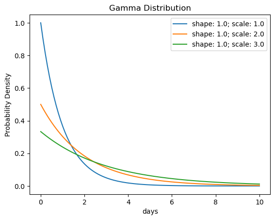
• As for the scale parameter, increasing its value results in a smoother probability curve of infection over time.

It is challenging to adjust the probability of infection directly by modifying the Gamma function, for example, by merely increasing or decreasing the probability.

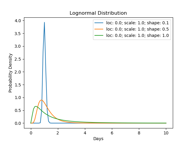
Moreover, we can adjust value of the infectiousness at its peak ~ max_infectiousness, which is usually represented by a lognormal function. The lognormal is determined by three factors, shift, loc and scale:

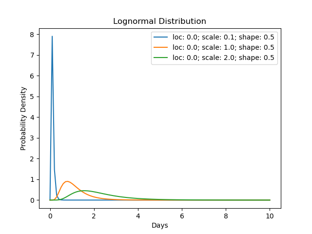
The final infection probability is calculated by max_infectiousness(t) * Gamma(t). In order to make the tuning simpler, we can use constant to represent max_infectiousness as well.

pobability_of_infection:
enable: true
adjust_factor:
   max_infectiousness:
     type: constant
     value: 10.0

In simpler terms, when we increased the frequency of interactions among individuals (represented by the contact matrix), we didn’t observe significant changes in terms of hospitalization and mortality rates. This is because the outcomes of the infection were not modified.

However, it’s important to note that in this experiment, the rate of exposure to the infection during the first 1-2 weeks was much higher compared to the baseline experiment.

Reduce the symptom cycle

The period of people expericing a symptom is determined by the symptom_trajectory.

We usually have the following trajectories:

• exposed => asymptomatic => recovered

• exposed => mild => recovered

• exposed => mild => severe => recovered

• exposed => mild => hospitalised => recovered

• exposed => mild => intensive_care => recovered

• exposed => mild => severe => dead

• exposed => mild => hospitalised => dead

• exposed => mild => hospitalised => intensive_care => dead

each stage of the symptom can be represented by different types of functions:

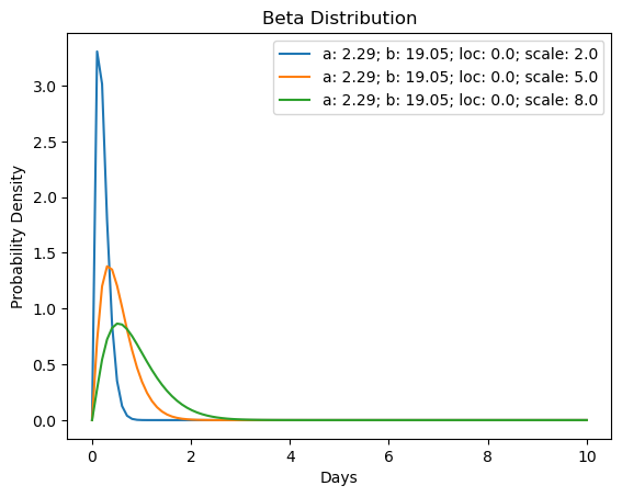
• beta (parameters: a, b, loc, scale)

• lognormal (parameters: shape, loc, scale)

• exponweib (parameters: a, c, loc, scale)

• constant

Now let’s check individual probability functions:

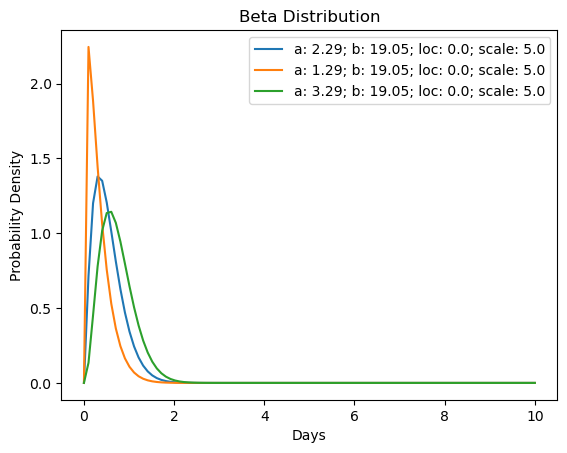
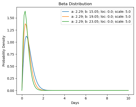
• For beta (as below):

  • when we increase a, the timing will increase

  • when we increase b, the timing will decrease

  • when we increase scale, the timing will increase

  

  

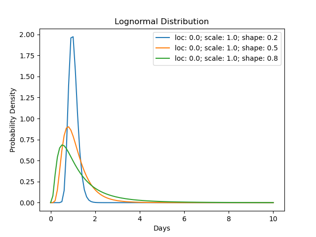
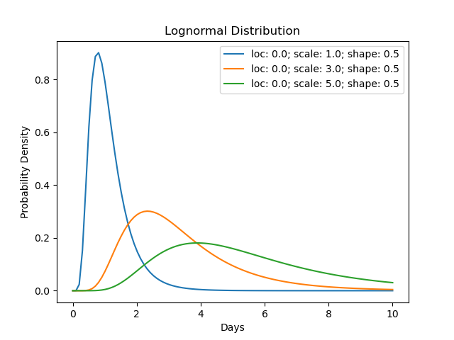
• For lognormal (as below):

  • when we increase shape, the timing will decrease

  • when we increase scale, the timing will increase

  

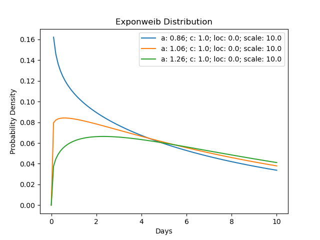
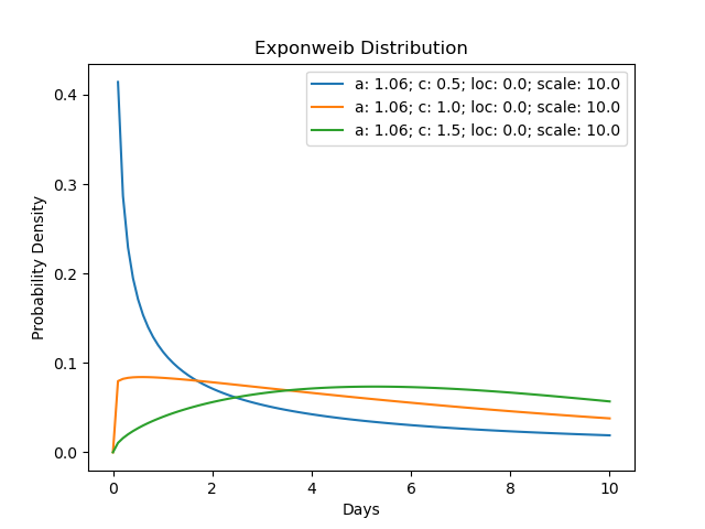
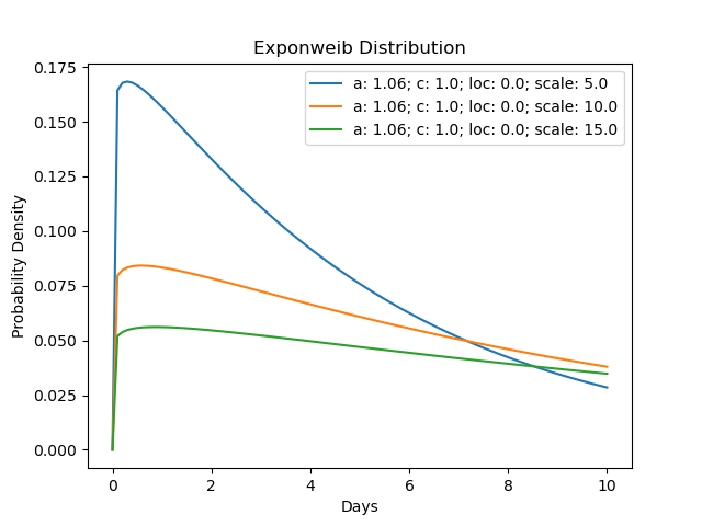
• For exponweib (as below):

  • when we increase a, the timing will decrease

  • when we increase c, the timing will increase

  • when we increase scale, the timing will increase

  

  

In order to tune the symptom trajectory, we can adjust the probability function in general, or target at a sepcfic trajectory.

symptom_trajectory:
enable: true
adjust_factor:
   general:
      beta:
      enable: true
      a: 1.0
      b: 1.0
      loc: 1.0
      scale: 0.3
      lognormal:
      enable: true
      s: 1.0
      loc: 1.0
      scale: 0.3
      exponweib:
      enable: true
      a: 1.0
      c: 1.0
      loc: 1.0
      scale: 0.3
   traj1:
      name: exposed => mild => severe => dead_home
      paras:
      - symptom_tag: exposed
         completion_time:
            type: beta
            a: 2.29
            b: 19.05
            loc: 0.39
            scale: 39.8

We can see that by reducing scale in the symptom trajectory, we can increase the symptom cycle easily.