Data
JUNE_NZ requires a number of input files.
The script cli_data.py is provided to create all the required inputs for JUNE_NZ.
cli_data --workdir <Working directory>
         --cfg <Data configuration>
         --scale <Population scale>
         --disease_cfg_dir <Disease configuration directory>
         --policy_cfg_path <Policy configuration path>
         [--exclude_super_areas A1, A2]
         [--use_sa3_as_super_area]
The command options are explained as below:
--workdir: Specifies the directory where the generated data will be stored. For example,--workdir /tmp/june_data.--cfg: Sets the configuration for retrieving the source data. For example,--cfg etc/june_data.yml.--scale: Determines the percentage of the population to be used. For instance, a value of 0.1 means only 10% of the population will be utilized. For example,--scale 0.1--exclude_super_areas: Allows excluding specific super areas from the model. For example,--exclude_super_areas A1 A2.--disease_cfg_dir: Disease configuration directory. For example,--disease_cfg_dir etc/cfg/disease/covid-19.--policy_cfg_path: Policy file. For example,--policy_cfg_path etc/cfg/policy/policy1.yaml.--simulation_cfg_path: Simulation file. For example,--simulation_cfg_path etc/cfg/simulation/simulation_cfg.yml.--use_sa3_as_super_area: If useSA3as super area level, otherwise we will use regional council as super area level. Note thatSA3is not a standard statistical level, therefore many information are aggregated fromSA2(e.g.,super_area_location).
Note
Most input data are created from raw dataset stored in June_NZ_data (most of them are obtained from NZ.Stat), while some inputs are defined via:
the fixed variable
FIXED_DATA(process/__init__.py), orfrom external configuration files:
Disease configuration (the directory contains all the information about the population disease, including the viruses we want to investigate), e.g.,
etc/cfg/disease/covid-19Policy configuration, e.g.,
etc/cfg/policy/policy1.yamlSimulation control configuration, e.g.,
etc/cfg/simulation/simulation_cfg.ymlVaccination configuration, e.g.,
etc/cfg/disease/vaccine/vaccine1.yaml
The following contents show different types of inputs for JUNE_NZ.
1. Population data (demography)
It defines the population (agents) to be used in the model.
Data |
Geography level |
Example |
|---|---|---|
The number of people (grouped by age) |
area |
age_profile.csv |
The number of people (grouped by age and ethnicities) |
area |
ethnicity_profile.csv |
The percentage of female (grouped by age) |
area |
gender_profile_female_ratio.csv |
Note
The number of people (grouped by age) determines the number of total people to be used in the model.
2. Geography data
It defines the geography (grid) to be used in the model.
Data |
Geography level |
Example |
|---|---|---|
Area latitude and longitude |
area |
area_location.csv |
Super area latitude and longitude |
super area |
super_area_location.csv |
Super area names |
super area |
supare_area_name.csv |
Super area and area socioeconomic_centile |
super area, area |
area_socialeconomic_index.csv |
Hierarchy of region, super area and area |
region, super area, area |
geography_hierarchy_definition.csv |
3. Group (activities) data
Group data contains different types of activities (e.g., company, household, hospital, school and leisure) that an individual might do every day.
3.1 Company
It defines the companies used in the model
Data |
Geography level |
Example |
|---|---|---|
Number of employers by firm size |
super area |
employers_by_firm_size.csv |
Number of employers by sector type |
super area |
sectors_by_sector.csv |
Number of employees by sector and age |
area |
employees.csv |
When company close, who will be the key worker etc. |
|
company_closure.yaml |
Sub-sector configuration |
|
subsector_cfg.yaml |
In the above data, Number of employers by firm size, Number of employers by sector type and Number of employees
are obtained from NZ.Stat, while company clousre and sub-sector configuration are defined in the variable FIXED_DATA. For example,
"company": {
    "employees": {"employment_rate": 0.7},
    "company_closure": {
        "company_closure": {
            "sectors": {
                "A": {"key_worker": 1.0, "furlough": 0.0, "random": 0.0},
                "P": {"key_worker": 0.0, "furlough": 0.0833, "random": 0.9167},
                ...
                "S": {"key_worker": 0.0, "furlough": 0.0, "random": 1.0},
            }
        }
    },
    "subsector_cfg": {
        "age_range": [18, 64],
        "sub_sector_ratio": {"P": {"m": 0.4, "f": 0.6}, "Q": {"m": 0.5, "f": 0.5}},
        "sub_sector_distr": {
            "P": {
                "label": ["teacher_secondary", "teacher_primary"],
                "m": [0.72526887, 0.27473113],
                "f": [0.72526887, 0.27473113],
            },
            ...
            "Q": {
                "label": ["doctor", "nurse"],
                "m": [0.65350126, 0.34649874],
                "f": [0.16103136, 0.83896864],
            },
        },
    },
},
Note
The Number of employees from NZStats somehome is smaller than the expected value compared to the NZ population. Therefore, in FIXED_DATA
we have a variable called employment_rate, which is a factor makes number of employees matches to the assumed number of people in employment.
3.2 Household
It defines the household information used in the model
Data |
Geography level |
Example |
|---|---|---|
Age difference for parents-children |
super area |
age_difference_parent_child.csv |
Age difference for couple |
super area |
age_difference_couple.csv |
Number of regular household (e.g., with different household composition) |
area |
household.csv |
Regular household defination |
|
household_def.yaml |
Number of communal household |
area |
household_commual.csv |
Number of student only household (e.g., dormitory) |
area |
household_student.csv |
The household information come from both external dataset and FIXED_DATA:
For example,
for setting up the age differences between couples and parents-children, we have:
FIXED_DATA = {
    "group": {
        ......
        "household": {
            "age_difference_couple": {
                "age_difference": [-5, 0, 5, 10],
                "frequency": [0.1, 0.7, 0.1, 0.1],
            },
            "age_difference_parent_child": {
                "age_difference": [25, 50],
                "0": [0.1, 0.9],
                "1": [0.1, 0.9],
                "2": [0.2, 0.8],
                "3": [0.3, 0.7],
                "4 or more": [0.3, 0.7],
            },
        },
    ...
where the above defines the assumed age differences for both couples and parents-children.
Note
The
number of householdare obtained from NZ.Stat. However there is a lack of detailed information, thus the only household type=0 >=0 >=0 >=0 >=0is used in the model.We also set the number of commnual and student househodls to zero, since the lack of detailed dataset.
3.3 Hospital
It defines the hospital information used in the model
Data |
Geography level |
Example |
|---|---|---|
Hospital information (address, number of beds/ICUs etc.) |
area |
hospitals.csv |
Hospital configuration (the age of worker in this sector etc.) |
|
hospital_config.yaml |
How many hospital (maximum) a person could visit |
|
neighbour_hospitals.yaml |
The information above include the hospital address (latitude and longitude), number of beds and number of ICU beds. Also some affiliated data for hospital, such as the the minimum age working in this sector, and the number of hospitals that an indiviual agent could visit.
3.4 School
It defines the school information used in the model
Data |
Geography level |
Example |
|---|---|---|
School information (address, student age range) |
area |
schools.csv |
The information would include the school address (latitude and longitude), and the student profile (e.g., min and max age)
3.5 Leisure (cinema, grocery, pub, gym and household visit)
It defines the leisure information used in the model
Data |
Geography level |
Example |
|---|---|---|
Cinema locations |
super area |
data/cinema.csv |
Cinema configuration (e.g., the chance that people may visit) |
|
data/cinema_cfg.yaml |
Grocery locations |
super area |
data/grocery.csv |
Grocery configuration (e.g., the chance that people may visit) |
|
cfg/grocery_cfg.yaml |
Gym locations |
super area |
data/gym.csv |
Gym configuration (e.g., the chance that people may visit) |
|
cfg/gym_cfg.yaml |
Pub locations |
super area |
data/pub.csv |
Pub configuration (e.g., the chance that people may visit) |
|
cfg/pub_cfg.yaml |
Household visit configuration |
|
cfg/household_visit_cfg.yaml |
The information would include all the leisure activities.
Note that all the location information are obtained from the Open Street Map, while all the configurations are from FIXED_DATA. For example, for cinema, we have:
"pub": {
        "times_per_week": {
            "weekday": {
                "male": {
                    "0-9": 0.032,
                    "9-15": 0.106,
                    ...
                    "86-100": 0.033,
                },
                "female": {
                    "0-9": 0.135,
                    ...,
                    "86-100": 0.02,
                },
            },
            "weekend": {
                "male": {
                    "0-9": 0.038,
                    ...
                    "86-100": 0.063,
                },
                "female": {
                    "0-9": 0.043,
                    ...
                    "86-100": 0.06,
                },
            },
        },
        "hours_per_day": {
            "weekday": {
                "male": {"0-65": 3, "65-100": 11},
                "female": {"0-65": 3, "65-100": 11},
            },
            "weekend": {"male": {"0-100": 12}, "female": {"0-100": 12}},
        },
        "drags_household_probability": 0,
        "neighbours_to_consider": 7,
        "maximum_distance": 10,
    },
The above shows how frequent a person might visit a cinema (over weekdays and weekends), how many different cinemas he/she might consider, and how long
he/she might travel (neighbours_to_consider, maximum_distance)to go to a cinema.
4. Commute
Commute defines how people move across different areas
Data |
Geography level |
Example |
|---|---|---|
How people travel (commute method) in different areas |
area |
transport_mode.csv |
Define if a travel method is public or not |
|
transport_def.yaml |
Number of inter-state stations |
super area |
number_of_inter_city_stations.yaml |
Seat-passanger ratio |
super area |
passage_seats_ratio.yaml |
How people travel across different super areas for work |
super area |
home_and_workplace.csv |
Note that transport_def.yaml is defined in the variable FIXED_DATA, e.g.,
FIXED_DATA = {
    ...
    "group": {
        "commute": {
            "transport_def": [
                {"description": "Work mainly at or from home", "is_public": False},
                {"description": "Underground, metro, light rail, tram", "is_public": True},

                ...

                {"description": "On foot", "is_public": False},
                {"description": "Other method of travel to work", "is_public": False},
            ]
        },
    ...
Note that when we use SA3 as the super_area, the Number of inter-state stations is dependant on the population in each SA3 ~ there will be one additional station
when the population increases by 5000. However, when we use New Zealand regions as the super_area, the number of stations is defined in FIXED_DATA.
5. Interaction
It defines the interaction intensity matrix for all the group members (e.g., school, hospital etc.)
Data |
Geography level |
Example |
|---|---|---|
Base interaction intensity and susceptibilities |
|
general.yaml |
Cinema interaction matrix |
|
cinema.csv |
Company interaction matrix |
|
company.csv |
Grocery interaction matrix |
|
grocery.csv |
Gym interaction matrix |
|
gym.csv |
Hospital interaction matrix |
|
hospital.csv |
Household interaction matrix |
|
household.csv |
Pub interaction matrix |
|
pub.csv |
School interaction matrix |
|
school.csv |
Commute (city_transport, and inter_city_transport) interaction matrix |
|
school.csv |
The above data are defined through FIXED_DATA.
(It is worthwhile to note that when the activity is household_visit, the contact matrix is borrowed from household therefore we don’t need a seperate household_visit contact matrix)
6. Disease data
Defines disease properties (population comorbidities, probability of infection, infection outcome, symtom trajectory, and virus intensity):
Data |
Geography level |
Example |
|---|---|---|
Comorbidities (prevalence) for female (grouped by age) |
|
comorbidities_female.csv |
Comorbidities (prevalence) for male (grouped by age) |
|
comorbidities_male.csv |
Comorbidities intensity |
|
comorbidity_intensity.yaml |
Probability of infection |
|
covid19.yaml |
Infection outcome (the ratio of symptoms) |
|
infection_outcome_ratio.csv |
Symptom trajectory timing profile |
|
symptom_trajectories.yaml |
Virus intensity |
|
virus_intensity.yaml |
6.1 Comorbidities
Comorbidities are defined by the variable FIXED_DATA, which is located in process/__init__.py. The comorbidity is one of the parameters determing the severity of symptom that
an individual may experience.
comorbidities_female: the ratio of female have certain comorbidities (grouped by ages)comorbidities_male: the ratio of male have certain comorbidities (grouped by ages)comorbidities_intensity: the intensity of the comorbidities
Note
For example, if the average female comorbidity intensity for the age group 50 is 1.02: tt is caculated by [0, 0.1, 0.9] * [0.8, 1.2, 1.0] where [0, 0.1, 0.9] is the
ratio of comorbidities and [0.8, 1.2, 1.0] represents the intensities of comorbidities.
If a person has disease2, which has the intensity of 1.2, then the symptom multiplier factor for this person is 1.2/1.02=1.18 which is larger than 1.0,
and therefore will lead to higher chance of experiencing severe symptoms.
An example of the defination of Comorbidities is:
"comorbidities_female": {
    "comorbidity": ["disease1", "disease2", "no_condition"],
    5: [0, 0, 1.0],
    10: [0, 0, 1.0],
    20: [0, 0, 1.0],
    50: [0, 0.1, 0.9],
    75: [0, 0.2, 0.8],
    100: [0.9, 0.0, 0.1],
},
"comorbidities_male": {
    "comorbidity": ["disease1", "disease2", "no_condition"],
    5: [0, 0, 1.0],
    10: [0, 0, 1.0],
    20: [0, 0, 1.0],
    50: [0, 0.1, 0.9],
    75: [0, 0.2, 0.8],
    100: [0.9, 0.0, 0.1],
},
"comorbidities_intensity": {"disease1": 0.8, "disease2": 1.2, "no_condition": 1.0},
6.2 Virus intensity
The virus intensity is a parameter that influences the severity of symptoms. As the intensity value increases, the likelihood of an individual experiencing more severe symptoms also increases. This can be achieved by elevating the probability of severe symptoms in addition to the ‘infection_outcome’ input data.”
An example of the virus intensity is:
Covid19: 1.3 # 170852960
B117: 1.5 # 37224668
B16172: 1.5 # 76677444
6.3 Symptom trajectory (infection outcome)
For the symptom trajectory, it is defined by a set of distribution functions (e.g., beta, log-normal etc.). Each distribution function comes with a set of parameters, those parameters decide the timeline for different symptoms during the infection.
The considered symptom stages include:
Recovered (-3)
Healthy (-2)
Exposed (-1)
Asymptomatic (0)
Mild (1)
Severe (2), which is calculated by
1.0 - [ Hospital + Die (from Home) + Asymptomatic + Mild]Hospital (3)
ICU (4)
Die (from home, 5)
Die (from hospital, 6)
Die (from ICU, 7)
For example, if we need to create a symptom trajectory for Die (from hospital, 6),
we need to go through the stages of Exposed (-1), Mild (1), Hospital (3) and Die (from hospital, 6) one by one.
Among this trajectory, at the stage of mild (-1), we create samples from a log-normal distribution with a specific, predefined parameters
(e.g., shape=0.55, loc=0.0, scale=5.0), a random number is drawn from these samples,
and it represents the timing for the infection (or we can understand it as the end time for the stage of symptom).
The chance of having a symptom is determined by:
Comorbidities (see the Section 4.1 of comorbidities for details)
Input infection outcome statistics (e.g., the percentage of symptoms that a person may experience, see Sectoin 4.3.1)
The target virus intnsity (see Section 4.2)
How long the sympton will last is dependant on:
The symptom trajectory (see Sectoin 4.3.2)
6.3.1 Input infection outcome statistics
An example of the infection outcome statistics is:
gp_asymptomatic_male |
gp_mild_male |
gp_ifr_male |
|
|---|---|---|---|
[0, 50] |
0.0 |
0.3 |
0.7 |
[51, 100] |
0.3 |
0.3 |
0.4 |
6.3.2 Symptom trajectory (infection outcome)
An example of the symptom trajectory is:
# exposed => mild => hospitalised => dead
- stages:
- symptom_tag: exposed
        completion_time:
        type: beta
        a: 2.29
        b: 19.05
        loc: 0.39
        scale: 39.8

- symptom_tag: mild
        completion_time:
        type: lognormal
        s: 0.55
        loc: 0.0
        scale: 5.

- symptom_tag: hospitalised
        completion_time:
        type: beta
        a: 1.21
        b: 1.97
        loc: 0.08
        scale: 12.9

- symptom_tag: dead_hospital
        completion_time:
        type: constant
        value: 0.
Note that the profile can be plotted using etc/test/plot_<profile>.py, where <profile> is the function name (e.g., beta, norm or lognorm).
6.4 Transmission profile
6.4.1 Base probability of infection
The transmssion profile determins the probability of the infection (e.g, the higher the probabilities, the more infectiousness an infector can be).
The probability of the infection is usually chosen from a Gamma profile, which is defined by (shape,shift,scale).
The following figures show the Gamma profile for different shape, shift (loc) and scale.
The x-axis is the value of shift (loc), which corresponds to the infection time. The y-axis is the probability of infection.
When a person is infected, the infection time will be applied to the above Gamma function (as x), and then obtain the related probability of infection.
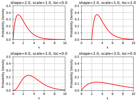
6.4.2 Adjust max infectiousness
The maximum infectiousness from the probability of infection is adjusted with the argument max_infectiousness. For an infector, a random
value will be drawn from the lognormal function, and it will be multiplied to the probability of function.
The lognormal is determined by parameters of shape, loc and scale.
For example, the following figures show the lognormal profile:

6.4.3 Adjust mild/asymptomatic infectiousness
We can adjust the the probability of infection based on a person’s maximum symptom. For example, if the maximum symtom is asymptomatic, we can
reduce the probability of infection profile by 50%.
An example for COVID-19 transmission is set up as:
type:
        'gamma'
shape:
        type: normal
        loc: 1.56
        scale: 0.08
rate:
        type: normal
        loc: 0.53
        scale: 0.03
shift:
        type: normal
        loc: -2.12
        scale: 0.1
asymptomatic_infectious_factor:
        type: constant
        value: 0.5
mild_infectious_factor:
        type: constant
        value: 1.
max_infectiousness:
        type: lognormal
        s: 0.5
        loc: 0.0
        scale: 1.
7. Vaccination data
The vaccine data must be specified if we want to simulate the effect of vaccination campaign in the model.
Data |
Geography level |
Example |
|---|---|---|
Vaccine features (age dependant) |
|
vaccine.yaml |